Warning: package 'tidyverse' was built under R version 4.4.3
Warning: package 'ggplot2' was built under R version 4.4.3
Warning: package 'tibble' was built under R version 4.4.3
── Attaching core tidyverse packages ──────────────────────── tidyverse 2.0.0 ──
✔ dplyr     1.1.4     ✔ readr     2.1.5
✔ forcats   1.0.0     ✔ stringr   1.5.1
✔ ggplot2   4.0.1     ✔ tibble    3.3.1
✔ lubridate 1.9.4     ✔ tidyr     1.3.1
✔ purrr     1.0.4
── Conflicts ────────────────────────────────────────── tidyverse_conflicts() ──
✖ dplyr::filter() masks stats::filter()
✖ dplyr::lag()    masks stats::lag()
ℹ Use the conflicted package (<http://conflicted.r-lib.org/>) to force all conflicts to become errors
library(dslabs)
Warning: package 'dslabs' was built under R version 4.4.3
library(dplyr)
#get an overview of data structurestr(gapminder)
'data.frame':   10545 obs. of  9 variables:
 $ country         : Factor w/ 185 levels "Albania","Algeria",..: 1 2 3 4 5 6 7 8 9 10 ...
 $ year            : int  1960 1960 1960 1960 1960 1960 1960 1960 1960 1960 ...
 $ infant_mortality: num  115.4 148.2 208 NA 59.9 ...
 $ life_expectancy : num  62.9 47.5 36 63 65.4 ...
 $ fertility       : num  6.19 7.65 7.32 4.43 3.11 4.55 4.82 3.45 2.7 5.57 ...
 $ population      : num  1636054 11124892 5270844 54681 20619075 ...
 $ gdp             : num  NA 1.38e+10 NA NA 1.08e+11 ...
 $ continent       : Factor w/ 5 levels "Africa","Americas",..: 4 1 1 2 2 3 2 5 4 3 ...
 $ region          : Factor w/ 22 levels "Australia and New Zealand",..: 19 11 10 2 15 21 2 1 22 21 ...
#get a summary of datasummary(gapminder)
                country           year      infant_mortality life_expectancy
 Albania            :   57   Min.   :1960   Min.   :  1.50   Min.   :13.20
 Algeria            :   57   1st Qu.:1974   1st Qu.: 16.00   1st Qu.:57.50
 Angola             :   57   Median :1988   Median : 41.50   Median :67.54
 Antigua and Barbuda:   57   Mean   :1988   Mean   : 55.31   Mean   :64.81
 Argentina          :   57   3rd Qu.:2002   3rd Qu.: 85.10   3rd Qu.:73.00
 Armenia            :   57   Max.   :2016   Max.   :276.90   Max.   :83.90
 (Other)            :10203                  NA's   :1453
   fertility       population             gdp               continent
 Min.   :0.840   Min.   :3.124e+04   Min.   :4.040e+07   Africa  :2907
 1st Qu.:2.200   1st Qu.:1.333e+06   1st Qu.:1.846e+09   Americas:2052
 Median :3.750   Median :5.009e+06   Median :7.794e+09   Asia    :2679
 Mean   :4.084   Mean   :2.701e+07   Mean   :1.480e+11   Europe  :2223
 3rd Qu.:6.000   3rd Qu.:1.523e+07   3rd Qu.:5.540e+10   Oceania : 684
 Max.   :9.220   Max.   :1.376e+09   Max.   :1.174e+13
 NA's   :187     NA's   :185         NA's   :2972
             region
 Western Asia   :1026
 Eastern Africa : 912
 Western Africa : 912
 Caribbean      : 741
 South America  : 684
 Southern Europe: 684
 (Other)        :5586
#determine what time of object gapminder isclass(gapminder)
[1] "data.frame"
#assign African countries to new object africadata <- gapminder %>%filter(continent =="Africa")#overview of data structurestr(africadata)
'data.frame':   2907 obs. of  9 variables:
 $ country         : Factor w/ 185 levels "Albania","Algeria",..: 2 3 18 22 26 27 29 31 32 33 ...
 $ year            : int  1960 1960 1960 1960 1960 1960 1960 1960 1960 1960 ...
 $ infant_mortality: num  148 208 187 116 161 ...
 $ life_expectancy : num  47.5 36 38.3 50.3 35.2 ...
 $ fertility       : num  7.65 7.32 6.28 6.62 6.29 6.95 5.65 6.89 5.84 6.25 ...
 $ population      : num  11124892 5270844 2431620 524029 4829291 ...
 $ gdp             : num  1.38e+10 NA 6.22e+08 1.24e+08 5.97e+08 ...
 $ continent       : Factor w/ 5 levels "Africa","Americas",..: 1 1 1 1 1 1 1 1 1 1 ...
 $ region          : Factor w/ 22 levels "Australia and New Zealand",..: 11 10 20 17 20 5 10 20 10 10 ...
#summary of data
summary(africadata)
         country          year      infant_mortality life_expectancy
 Algeria     :  57   Min.   :1960   Min.   : 11.40   Min.   :13.20
 Angola      :  57   1st Qu.:1974   1st Qu.: 62.20   1st Qu.:48.23
 Benin       :  57   Median :1988   Median : 93.40   Median :53.98
 Botswana    :  57   Mean   :1988   Mean   : 95.12   Mean   :54.38
 Burkina Faso:  57   3rd Qu.:2002   3rd Qu.:124.70   3rd Qu.:60.10
 Burundi     :  57   Max.   :2016   Max.   :237.40   Max.   :77.60
 (Other)     :2565                  NA's   :226
   fertility       population             gdp               continent
 Min.   :1.500   Min.   :    41538   Min.   :4.659e+07   Africa  :2907
 1st Qu.:5.160   1st Qu.:  1605232   1st Qu.:8.373e+08   Americas:   0
 Median :6.160   Median :  5570982   Median :2.448e+09   Asia    :   0
 Mean   :5.851   Mean   : 12235961   Mean   :9.346e+09   Europe  :   0
 3rd Qu.:6.860   3rd Qu.: 13888152   3rd Qu.:6.552e+09   Oceania :   0
 Max.   :8.450   Max.   :182201962   Max.   :1.935e+11
 NA's   :51      NA's   :51          NA's   :637
                       region
 Eastern Africa           :912
 Western Africa           :912
 Middle Africa            :456
 Northern Africa          :342
 Southern Africa          :285
 Australia and New Zealand:  0
 (Other)                  :  0
#create new object from africadata that has only infant_mortality and life_expectancy africa_inf_exp <- africadata %>%select("infant_mortality", "life_expectancy")#create new object from africadata that has only population and life_expectancyafrica_pop_exp <- africadata %>%select("population", "life_expectancy")#structure overview of both africa_inf_exp and africa_pop_expstr(africa_inf_exp)
'data.frame':   2907 obs. of  2 variables:
 $ infant_mortality: num  148 208 187 116 161 ...
 $ life_expectancy : num  47.5 36 38.3 50.3 35.2 ...
str(africa_pop_exp)
'data.frame':   2907 obs. of  2 variables:
 $ population     : num  11124892 5270844 2431620 524029 4829291 ...
 $ life_expectancy: num  47.5 36 38.3 50.3 35.2 ...
#summary of both
summary(africa_inf_exp)
 infant_mortality life_expectancy
 Min.   : 11.40   Min.   :13.20
 1st Qu.: 62.20   1st Qu.:48.23
 Median : 93.40   Median :53.98
 Mean   : 95.12   Mean   :54.38
 3rd Qu.:124.70   3rd Qu.:60.10
 Max.   :237.40   Max.   :77.60
 NA's   :226
summary(africa_pop_exp)
   population        life_expectancy
 Min.   :    41538   Min.   :13.20
 1st Qu.:  1605232   1st Qu.:48.23
 Median :  5570982   Median :53.98
 Mean   : 12235961   Mean   :54.38
 3rd Qu.: 13888152   3rd Qu.:60.10
 Max.   :182201962   Max.   :77.60
 NA's   :51
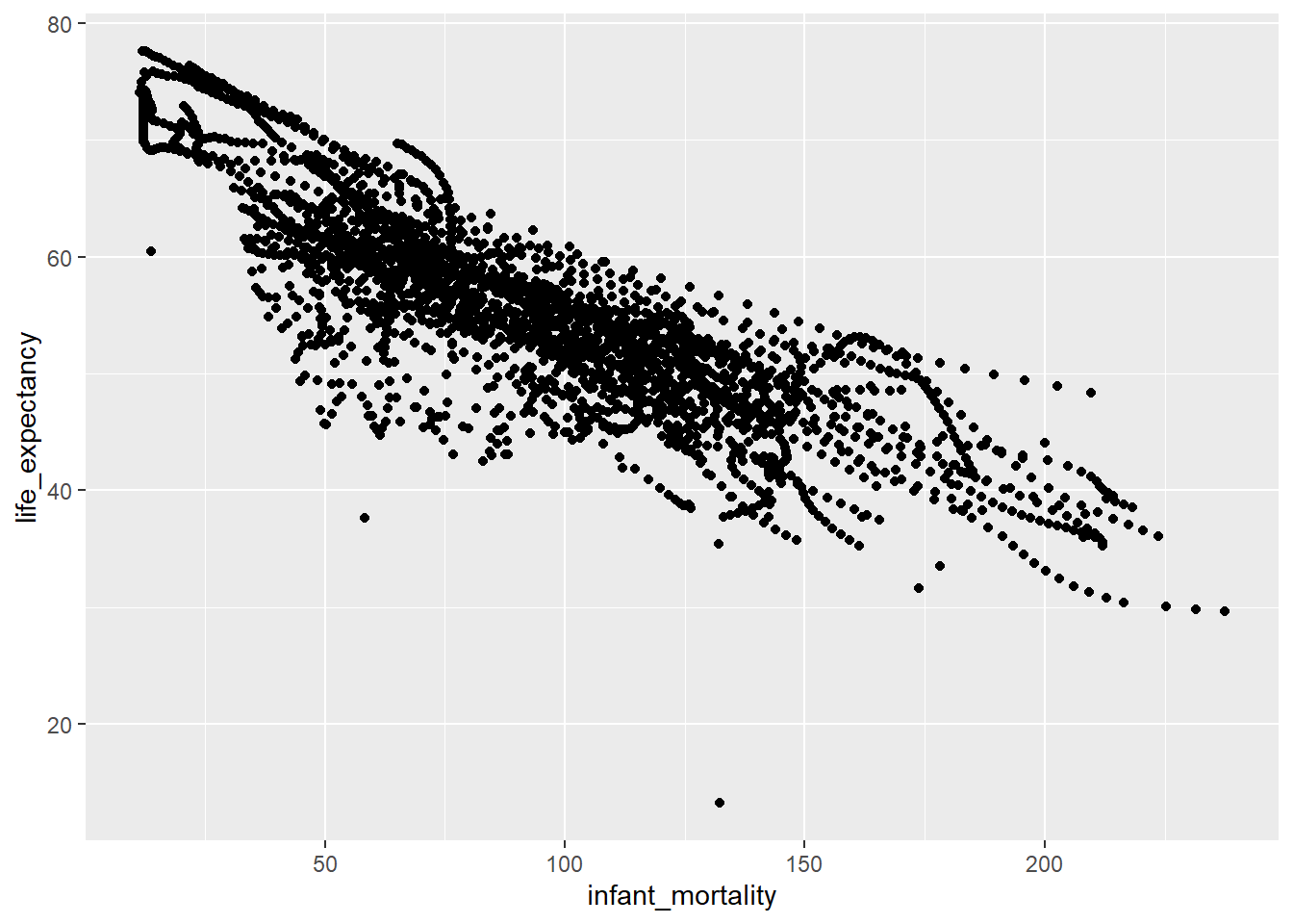
#plot infant_mortality (x) vs. life_expectancy (y)ggplot(africa_inf_exp, (aes(x = infant_mortality, y = life_expectancy))) +geom_point()
Warning: Removed 226 rows containing missing values or values outside the scale range
(`geom_point()`).
#plot population (x) vs. life expectancy (y)##population in log scale so log(x) vs. (y)###check structureafrica_pop_exp <- africa_pop_exp %>%mutate(log_population =log10(population))str(africa_pop_exp)
'data.frame':   2907 obs. of  3 variables:
 $ population     : num  11124892 5270844 2431620 524029 4829291 ...
 $ life_expectancy: num  47.5 36 38.3 50.3 35.2 ...
 $ log_population : num  7.05 6.72 6.39 5.72 6.68 ...
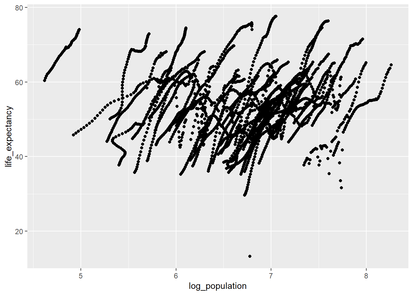
ggplot(africa_pop_exp, (aes(x = log_population, y = life_expectancy))) +geom_point()
Warning: Removed 51 rows containing missing values or values outside the scale range
(`geom_point()`).
Appearance of streaks - likely represent each country over time as its population and life expextancy both slowly increase.
#identify where the NA values are, to avoid them in the next step missing_inf_years <- africadata %>%filter(is.na(infant_mortality)) %>%pull(year) %>%unique()#new object with only year 2000 data africadata_2000 <- africadata %>%filter(year ==2000)#structure of new africa_data2000str(africadata_2000)
'data.frame':   51 obs. of  9 variables:
 $ country         : Factor w/ 185 levels "Albania","Algeria",..: 2 3 18 22 26 27 29 31 32 33 ...
 $ year            : int  2000 2000 2000 2000 2000 2000 2000 2000 2000 2000 ...
 $ infant_mortality: num  33.9 128.3 89.3 52.4 96.2 ...
 $ life_expectancy : num  73.3 52.3 57.2 47.6 52.6 46.7 54.3 68.4 45.3 51.5 ...
 $ fertility       : num  2.51 6.84 5.98 3.41 6.59 7.06 5.62 3.7 5.45 7.35 ...
 $ population      : num  31183658 15058638 6949366 1736579 11607944 ...
 $ gdp             : num  5.48e+10 9.13e+09 2.25e+09 5.63e+09 2.61e+09 ...
 $ continent       : Factor w/ 5 levels "Africa","Americas",..: 1 1 1 1 1 1 1 1 1 1 ...
 $ region          : Factor w/ 22 levels "Australia and New Zealand",..: 11 10 20 17 20 5 10 20 10 10 ...
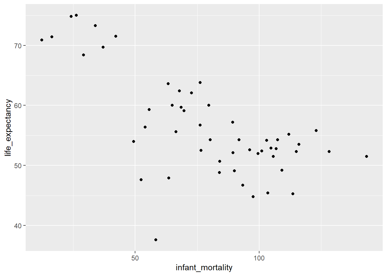
#plot infant_mortality (x) vs. life_expectancy (y)ggplot(africadata_2000, (aes(x = infant_mortality, y = life_expectancy))) +geom_point()
##plot population (x) vs. life expectancy (y)##population in log scale so log(x) vs. (y)###check structureafricadata_2000 <- africadata_2000 %>%mutate(log_population =log10(population))str(africadata_2000)
'data.frame':   51 obs. of  10 variables:
 $ country         : Factor w/ 185 levels "Albania","Algeria",..: 2 3 18 22 26 27 29 31 32 33 ...
 $ year            : int  2000 2000 2000 2000 2000 2000 2000 2000 2000 2000 ...
 $ infant_mortality: num  33.9 128.3 89.3 52.4 96.2 ...
 $ life_expectancy : num  73.3 52.3 57.2 47.6 52.6 46.7 54.3 68.4 45.3 51.5 ...
 $ fertility       : num  2.51 6.84 5.98 3.41 6.59 7.06 5.62 3.7 5.45 7.35 ...
 $ population      : num  31183658 15058638 6949366 1736579 11607944 ...
 $ gdp             : num  5.48e+10 9.13e+09 2.25e+09 5.63e+09 2.61e+09 ...
 $ continent       : Factor w/ 5 levels "Africa","Americas",..: 1 1 1 1 1 1 1 1 1 1 ...
 $ region          : Factor w/ 22 levels "Australia and New Zealand",..: 11 10 20 17 20 5 10 20 10 10 ...
 $ log_population  : num  7.49 7.18 6.84 6.24 7.06 ...
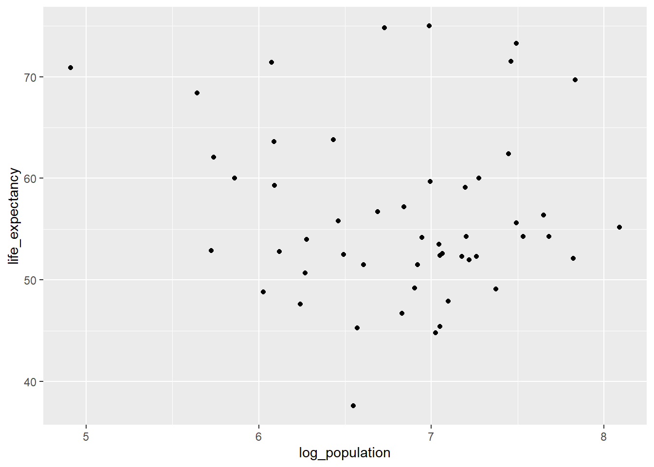
ggplot(africadata_2000, (aes(x = log_population, y = life_expectancy))) +geom_point()
#Fit life expectancy as the outcome, and infant mortality as the predictorfit1 <-lm(life_expectancy ~ infant_mortality, data = africadata_2000)#Fit life expectancy as the outcome, and population as the predictorfit2 <-lm(life_expectancy ~ population, data = africadata_2000)#I wasn't sure if you wanted population or the log_population, so I did fit3 to be the log_populationfit3 <-lm(life_expectancy ~ log_population, data = africadata_2000)#summary of the fits summary(fit1)
Call:
lm(formula = life_expectancy ~ infant_mortality, data = africadata_2000)

Residuals:
     Min       1Q   Median       3Q      Max
-22.6651  -3.7087   0.9914   4.0408   8.6817

Coefficients:
                 Estimate Std. Error t value Pr(>|t|)
(Intercept)      71.29331    2.42611  29.386  < 2e-16 ***
infant_mortality -0.18916    0.02869  -6.594 2.83e-08 ***
---
Signif. codes:  0 '***' 0.001 '**' 0.01 '*' 0.05 '.' 0.1 ' ' 1

Residual standard error: 6.221 on 49 degrees of freedom
Multiple R-squared:  0.4701,    Adjusted R-squared:  0.4593
F-statistic: 43.48 on 1 and 49 DF,  p-value: 2.826e-08
summary(fit2)
Call:
lm(formula = life_expectancy ~ population, data = africadata_2000)

Residuals:
    Min      1Q  Median      3Q     Max
-18.429  -4.602  -2.568   3.800  18.802

Coefficients:
             Estimate Std. Error t value Pr(>|t|)
(Intercept) 5.593e+01  1.468e+00  38.097   <2e-16 ***
population  2.756e-08  5.459e-08   0.505    0.616
---
Signif. codes:  0 '***' 0.001 '**' 0.01 '*' 0.05 '.' 0.1 ' ' 1

Residual standard error: 8.524 on 49 degrees of freedom
Multiple R-squared:  0.005176,  Adjusted R-squared:  -0.01513
F-statistic: 0.2549 on 1 and 49 DF,  p-value: 0.6159
summary(fit3)
Call:
lm(formula = life_expectancy ~ log_population, data = africadata_2000)

Residuals:
    Min      1Q  Median      3Q     Max
-19.113  -4.809  -1.554   3.907  18.863

Coefficients:
               Estimate Std. Error t value Pr(>|t|)
(Intercept)      65.324     12.520   5.217 3.65e-06 ***
log_population   -1.315      1.829  -0.719    0.476
---
Signif. codes:  0 '***' 0.001 '**' 0.01 '*' 0.05 '.' 0.1 ' ' 1

Residual standard error: 8.502 on 49 degrees of freedom
Multiple R-squared:  0.01044,   Adjusted R-squared:  -0.009755
F-statistic: 0.517 on 1 and 49 DF,  p-value: 0.4755
What I found here - fit1: p-value = 2.826e-08, R-squared = 0.4593 - p-value indicates significant difference (well below 0.05), but with an R-squared of 0.4593, that is ia fairly weak inverse (negative) correlation between life expectancy and infant mortality, confirmed visually with plot fit2: p-value = 0.6159, R-squared = -0.01513 - p-value indicates no significant difference (above 0.05), no relationship between life_expectancy and population fit3: p-vlaue = 0.4755, R-squared = -0.009755 - p-value indicates no signifiicant difference (above 0.05), no relationhsip between life expectancy and log_population
Additional exploration: dslabs::gapminder (contributed by Alexandra Tejada-Strop)
In this section I explore the gapminder dataset from the dslabs package. I do basic exploration, some light cleaning, a few figures, and then fit a simple regression model to describe how life expectancy relates to economic output and time.
Load packages —-
library(tidyverse) library(dslabs)
Load data —-
data(gapminder) # loads a data frame called gapminder
I create a few helpful variables: - gdp_per_cap: GDP per capita - log_gdp_per_cap: log10 GDP per capita (often more linear for modeling) I also remove rows where GDP or population are missing or zero (to avoid dividing by zero and taking log of non-positive values).
Relationship between life expectancy and GDP per capita (log scale), colored by region
1) Life expectancy over time by region
gap2 %>% group_by(year, region) %>% summarise(mean_life_exp = mean(life_expectancy), .groups = “drop”) %>% ggplot(aes(x = year, y = mean_life_exp, color = region)) + geom_line() + labs( title = “Average life expectancy over time by region”, x = “Year”, y = “Average life expectancy” )
2) Life expectancy vs GDP per cap (log scale)
gap2 %>% ggplot(aes(x = log_gdp_per_cap, y = life_expectancy, color = region)) + geom_point(alpha = 0.4) + geom_smooth(method = “lm”, se = FALSE) + labs( title = “Life expectancy vs log10(GDP per capita)”, x = “log10(GDP per capita)”, y = “Life expectancy” )
Simple statistical model
I fit a linear regression model predicting life expectancy from: - log10(GDP per capita) - year (to capture general time trends) - region (to capture broad geographic differences)
This is not meant to be causal, just a simple descriptive model.
m1 <- lm(life_expectancy ~ log_gdp_per_cap + year + region, data = gap2) summary(m1)
A cleaner coefficient table
broom::tidy(m1) %>% arrange(p.value)
Results (plain-language summary)
The coefficient for log_gdp_per_cap is typically positive: higher GDP per capita is associated with higher life expectancy.
The coefficient for year is typically positive: life expectancy tends to increase over time.
Regional coefficients reflect systematic differences across regions after accounting for GDP per capita and time.
(Exact estimates may vary slightly depending on filtering and package versions.)